Seismic Receiver Function Inversion#
Receiver functions are a common observable in seismology. They represent the conversion of the form of energy of seismic waves from compressional to transverse (and vice versa) at geological interfaces. Details aside, the aim of a receiver function inversion is to determine the seismic structure at a point down to a depth of a few tens of kilometers. Typically the subsurface is parameterised as a few layers of constant velocity, where the thickness, velocity (and potentially even number) of layers are unknowns to be solved for.
This example uses the espresso library to provide data, a forward solver and other utilities related to a receiver function inversion.
from espresso import ReceiverFunctionInversion
import numpy as np
import matplotlib.pyplot as plt

from neighpy import NASearcher, NAAppraiser
Set up Espresso Receiver Function Inversion#
We start with a problem where we want to find the seismic velocity in fixed layers.
rfi = ReceiverFunctionInversion(example_number=2)
rfi.description
'Inverting velocities of 5 layers'
Lets have a look at the data
rfi.plot_data(rfi.data)
<Axes: xlabel='Time/s', ylabel='Amplitude'>

To first order, every peak in the receiver function is caused by a seismic discontinuity (change in seismic velocity).
And now let’s look at what a “good” model looks like, and a potential starting model
ax = rfi.plot_model(rfi.good_model, rfi.starting_model, "Good model", "Starting model")
ax.legend()
<matplotlib.legend.Legend at 0x28307fa50>

Out of curiosity, let’s see how well these models fit the observed data
ax = rfi.plot_data(rfi.data, label="Data")
for name, (model, colour) in {"Starting model" : [rfi.starting_model, "r"], "Good model": [rfi.good_model, "b"]}.items():
    synth = rfi.forward(model)
    ax.plot(rfi._t, synth, label=name, c=colour)
ax.legend()
<matplotlib.legend.Legend at 0x283068cd0>

Set up Neighbourhood Algorithm with Neighpy#
Espresso provides us with a log_likelihood function, which we can use as our objective function (although remember to multiply by -1 since we want to minimise the objective!).
We can choose the bounds on the velocity in each layer as we wish.
These should be generally increasing with depth.
searcher = NASearcher(
    objective=lambda m: -1 * rfi.log_likelihood(rfi.data, rfi.forward(m)),
    bounds=[(3.5, 7.0)] * rfi.model_size,
    ni=2000,  # size of initial population
    ns=50,  # number of new samples at each iteration
    nr=10,  # number of neighbourhoods to resample at each iteration
    n=100  # number of iterations
)

searcher.run(parallel=False)  # some serialisation issues with the EspressoProblem object preventing parallelisation

best_i = np.argmin(searcher.objectives)
best = searcher.samples[best_i]
NAI - Initial Random Search
NAI - Optimisation Loop: 100%|██████████| 100/100 [00:08<00:00, 12.38it/s]
A rather crude check on the convergence
plt.plot(searcher.objectives, marker=".", linestyle="", markersize=2)
plt.scatter(best_i, searcher.objectives[best_i], c="g", s=10, zorder=10)
plt.axvline(searcher.ni, c="k", ls="--")
plt.yscale("log")
plt.text(0.05, 0.95, "Initial Random Search", transform=plt.gca().transAxes, ha="left")
plt.text(0.95, 0.95, "Neighbourhood Search", transform=plt.gca().transAxes, ha="right")
Text(0.95, 0.95, 'Neighbourhood Search')

Plot models
def _plot_model(model):
    model_setup = rfi._model_setup(model)
    px = np.zeros([2 * len(model_setup), 2])
    px[0::2, 0] = model_setup[:, 1]
    px[1::2, 0] = model_setup[:, 1]
    px[1::2, 1] = model_setup[:, 0]
    px[2::2, 1] = model_setup[:-1, 0]
    return px


ax = rfi.plot_model(
    rfi.good_model,
    label="Good model",
)
for model in searcher.samples[:searcher.ni]:
    ax.plot(*_plot_model(model).T, c="k", alpha=0.01)
ax.plot(
    *_plot_model(searcher.samples[np.argmin(searcher.objectives)]).T,
    "g--",
    label="Best model found"
)
ax.legend(loc="lower left")
<matplotlib.legend.Legend at 0x284457ed0>

Plot predicted data
ax = rfi.plot_data(rfi.data, label="Data")
_ylim = ax.get_ylim()
for model in searcher.samples[:searcher.ni]:
    ax.plot(rfi._t, rfi.forward(model), c="k", alpha=0.01)
ax.get_lines()[0].set_zorder(10)
ax.plot(rfi._t, rfi.forward(best), "g--", label="Best model found", zorder=11)
ax.set_ylim(_ylim)
ax.legend()
<matplotlib.legend.Legend at 0x289946250>

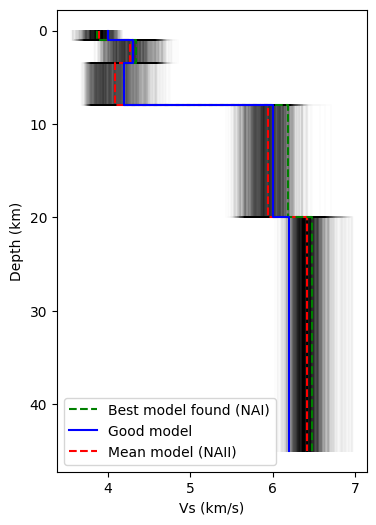
Pretty decent! Now to independently resample the posterior using the Appraisal phase of the NA.
appraiser = NAAppraiser(searcher=searcher, n_resample=20000, n_walkers=10)
appraiser.run()
NAII - Random Walk: 100%|██████████| 2000/2000 [00:43<00:00, 46.13it/s]
NAII - Random Walk: 100%|██████████| 2000/2000 [00:43<00:00, 46.11it/s]
NAII - Random Walk: 100%|██████████| 2000/2000 [00:43<00:00, 46.04it/s]
NAII - Random Walk: 100%|██████████| 2000/2000 [00:43<00:00, 46.01it/s]
NAII - Random Walk: 100%|██████████| 2000/2000 [00:43<00:00, 45.95it/s]
NAII - Random Walk: 100%|██████████| 2000/2000 [00:43<00:00, 45.94it/s]
NAII - Random Walk: 100%|██████████| 2000/2000 [00:43<00:00, 45.88it/s]
NAII - Random Walk: 100%|██████████| 2000/2000 [00:43<00:00, 45.85it/s]
NAII - Random Walk: 100%|██████████| 2000/2000 [00:43<00:00, 45.61it/s]
NAII - Random Walk: 100%|██████████| 2000/2000 [00:43<00:00, 45.54it/s]
ax = rfi.plot_model(best, rfi.good_model, label="Best model found (NAI)", label2="Good model")
for model in appraiser.samples[::10]:
    ax.plot(*_plot_model(model).T, c="k", alpha=0.01)
ax.get_lines()[0].set_color("g")
ax.get_lines()[0].set_linestyle("--")
ax.get_lines()[0].set_zorder(10)
ax.get_lines()[1].set_zorder(10)
ax.get_lines()[1].set_color("b")
ax.plot(*_plot_model(appraiser.mean).T, "r--", label="Mean model (NAII)")
ax.legend(loc="lower left")
<matplotlib.legend.Legend at 0x296ed6250>
fig, ax = plt.subplots(rfi.model_size, rfi.model_size, figsize=(10, 10), tight_layout=True)
for i in range(rfi.model_size):
    for j in range(rfi.model_size):
        ax[i, j].set_xlim(searcher.bounds[j])
        if i == j:
            ax[i, j].hist(appraiser.samples[:, j], bins=100, histtype="step", color="k")
            ax[i, j].axvline(best[j], c="g", ls="--")
            ax[i, j].axvline(rfi.good_model[j], c="b", ls="--")
            ax[i, j].axvline(appraiser.mean[j], c="r", ls="--")
        elif j<i:
            ax[i, j].scatter(appraiser.samples[:, j], appraiser.samples[:, i], s=1, c="k", alpha=0.01)
            ax[i, j].scatter(best[j], best[i], c="g", s=10, zorder=10)
            ax[i, j].scatter(rfi.good_model[j], rfi.good_model[i], c="b", s=10, zorder=10)
            ax[i, j].scatter(appraiser.mean[j], appraiser.mean[i], c="r", s=10, zorder=10)
        else:
            ax[i, j].axis("off")

A more complicated inversion#
What if we also wanted to invert for the interface depths?
rfi = ReceiverFunctionInversion(example_number=3)
rfi.description
'Inverting depths and velocities of 5 layers'
searcher = NASearcher(
    objective=lambda m: -1 * rfi.log_likelihood(rfi.data, rfi.forward(m)),
    bounds=[(0.1, 2), (3.5, 7.0),
            (0.5, 5), (3.5, 7.0),
            (2, 15), (3.5, 7.0),
            (10, 25), (3.5, 7.0),
            (15, 50), (3.5, 7.0),],
    ni=5000,  # size of initial population
    ns=200,  # number of new samples at each iteration
    nr=50,  # number of neighbourhoods to resample at each iteration
    n=100  # number of iterations
)

searcher.run(parallel=False)  # some serialisation issues with the EspressoProblem object preventing parallelisation

best_i = np.argmin(searcher.objectives)
best = searcher.samples[best_i]
NAI - Initial Random Search
NAI - Optimisation Loop: 100%|██████████| 100/100 [01:03<00:00, 1.57it/s]
plt.plot(searcher.objectives, marker=".", linestyle="", markersize=2)
plt.scatter(best_i, searcher.objectives[best_i], c="g", s=10, zorder=10)
plt.axvline(searcher.ni, c="k", ls="--")
plt.yscale("log")
plt.text(0.05, 0.95, "Initial Random Search", transform=plt.gca().transAxes, ha="left")
plt.text(0.95, 0.95, "Neighbourhood Search", transform=plt.gca().transAxes, ha="right")
Text(0.95, 0.95, 'Neighbourhood Search')

appraiser = NAAppraiser(searcher=searcher, n_resample=75000, n_walkers=15)
appraiser.run()
NAII - Random Walk: 100%|██████████| 5000/5000 [25:32<00:00,  3.26it/s]
NAII - Random Walk: 100%|██████████| 5000/5000 [25:33<00:00,  3.26it/s]
NAII - Random Walk: 100%|██████████| 5000/5000 [25:40<00:00,  3.25it/s]0:42,  3.82it/s]
NAII - Random Walk: 100%|██████████| 5000/5000 [25:42<00:00,  3.24it/s]
NAII - Random Walk: 100%|██████████| 5000/5000 [25:43<00:00,  3.24it/s]
NAII - Random Walk: 100%|██████████| 5000/5000 [25:44<00:00,  3.24it/s]
NAII - Random Walk: 100%|██████████| 5000/5000 [25:46<00:00,  3.23it/s]
NAII - Random Walk: 100%|██████████| 5000/5000 [25:48<00:00,  3.23it/s]
NAII - Random Walk: 100%|██████████| 5000/5000 [25:50<00:00,  3.22it/s]
NAII - Random Walk: 100%|██████████| 5000/5000 [25:51<00:00,  3.22it/s]
NAII - Random Walk: 100%|██████████| 5000/5000 [25:53<00:00,  3.22it/s]
NAII - Random Walk: 100%|██████████| 5000/5000 [25:53<00:00,  3.22it/s]
NAII - Random Walk: 100%|██████████| 5000/5000 [25:57<00:00,  3.21it/s]
NAII - Random Walk: 100%|██████████| 5000/5000 [25:58<00:00,  3.21it/s]
NAII - Random Walk: 100%|██████████| 5000/5000 [25:58<00:00,  3.21it/s]
ax = rfi.plot_model(best, rfi.good_model, label="Best model found (NAI)", label2="Good model")
for model in appraiser.samples[::10]:
    ax.plot(*_plot_model(model).T, c="k", alpha=0.01)
ax.get_lines()[0].set_color("g")
ax.get_lines()[0].set_linestyle("--")
ax.get_lines()[0].set_zorder(10)
ax.get_lines()[1].set_zorder(10)
ax.get_lines()[1].set_color("b")
ax.plot(*_plot_model(appraiser.mean).T, "r--", label="Mean model (NAII)")
ax.legend(loc="lower left")
<matplotlib.legend.Legend at 0x299af7ed0>

fig, ax = plt.subplots(rfi.model_size, rfi.model_size, figsize=(10, 10), tight_layout=True, gridspec_kw={"hspace": 0, "wspace": 0})
for i in range(rfi.model_size):
    for j in range(rfi.model_size):
        ax[i, j].set_xlim(searcher.bounds[j])
        ax[i, j].set_xticks([], [])
        ax[i, j].set_yticks([], [])
        if i == j:
            ax[i, j].hist(appraiser.samples[::10, j], bins=100, histtype="step", color="k")
            ax[i, j].axvline(best[j], c="g", ls="--")
            ax[i, j].axvline(rfi.good_model[j], c="b", ls="--")
            ax[i, j].axvline(appraiser.mean[j], c="r", ls="--")
        elif j<i:
            ax[i, j].scatter(appraiser.samples[::10, j], appraiser.samples[::10, i], s=1, c="k", alpha=0.01)
            ax[i, j].scatter(best[j], best[i], c="g", s=10, zorder=10)
            ax[i, j].scatter(rfi.good_model[j], rfi.good_model[i], c="b", s=10, zorder=10)
            ax[i, j].scatter(appraiser.mean[j], appraiser.mean[i], c="r", s=10, zorder=10)
            ax[i, j].set_ylim(searcher.bounds[i])
        else:
            ax[i, j].axis("off")

for ax_, xlabel in zip(ax[-1, :], ["d_1", "v_1", "d_2", "v_2", "d_3", "v_3", "d_4", "v_4", "d_5", "v_5"]):
    ax_.set_xlabel(xlabel)
for ax_, ylabel in zip(ax.T[0, :], ["d_1", "v_1", "d_2", "v_2", "d_3", "v_3", "d_4", "v_4", "d_5", "v_5"]):
    ax_.set_ylabel(ylabel)
ax[0,0].set_ylabel("")
Text(0, 0.5, '')

ax = rfi.plot_data(rfi.data, label="Data")
_ylim = ax.get_ylim()
for model in appraiser.samples[::15]:
    ax.plot(rfi._t, rfi.forward(model), c="k", alpha=0.01)
ax.get_lines()[0].set_zorder(10)
ax.plot(rfi._t, rfi.forward(best), "g--", label="Best model (I)", zorder=11)
ax.plot(rfi._t, rfi.forward(appraiser.mean), "r--", label="Mean model (II)", zorder=11)
ax.set_ylim(_ylim)
ax.legend()
<matplotlib.legend.Legend at 0x2c84efed0>
