Regression#
Simply fit some noisy data using the Neighbourhooc Algorithm.
import numpy as np
from scipy.spatial import Voronoi, voronoi_plot_2d
import matplotlib.pyplot as plt

from neighpy import NASearcher, NAAppraiser
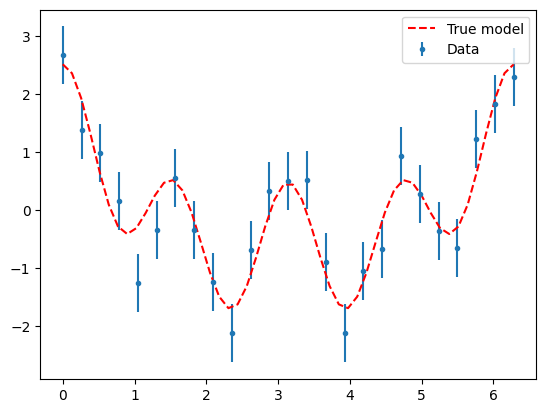
Create some noisy data. This will be a sum of cosines with a small amount of Gaussian noise.
rng = np.random.default_rng(42)
domain = (0, 2 * np.pi)
n_x = 50
x = np.linspace(*domain, num=n_x)
xm = np.linspace(*domain, num=n_x // 2)

def cosine(m, mask=True):
    _x = xm if mask else x
    _x = np.stack([i * _x for i in range(1, m.size + 1)])
    return np.sum(m[:, np.newaxis] * np.cos(_x), axis=0)
true_parameters = np.array([1, 0.5, 0.02, 1])
data = cosine(true_parameters)
sigma = 0.5
Cdinv = (1 / sigma ** 2) * np.eye(data.size)
data += rng.normal(loc=0, scale=sigma, size=data.shape)
plt.errorbar(xm, data, yerr=sigma, fmt=".", label="Data")
plt.plot(x, cosine(true_parameters, mask=False), "r--", label="True model")
plt.legend()
<matplotlib.legend.Legend at 0x11e852b90>
The objective function will be to minimise the error-weighted squared data misfit
def objective(m):
    prediction = cosine(m)
    residual = data - prediction
    return residual @ (Cdinv @ residual)
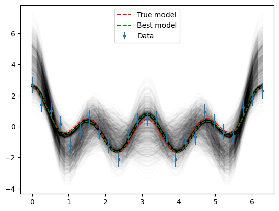
NA Direct Seach Phase#
After an initial random search of the parameter space, this phase iteratively resamples the “neighbourhoods” of the lowest-misfit regions. The result is a set of points, which when represented as a Voronoi diagram approximates the objective surface.
searcher = NASearcher(
    objective=objective,
    ns=100,
    nr=10,
    ni=1000,
    n=20,
    bounds=[(0, 2)] * 4,
)

searcher.run()
NAI - Initial Random Search
NAI - Optimisation Loop: 100%|██████████| 20/20 [00:00<00:00, 21.71it/s]
best = searcher.samples[np.argmin(searcher.objectives)]

plt.plot(x, np.apply_along_axis(cosine, 1, searcher.samples, mask=False).T, "k", alpha=0.01)
plt.errorbar(xm, data, yerr=sigma, fmt=".", label="Data")
plt.plot(x, cosine(true_parameters, mask=False), "r--", label="True model")
plt.plot(x, cosine(best, mask=False), "g--", label="Best model")
plt.legend()
<matplotlib.legend.Legend at 0x11f49e510>
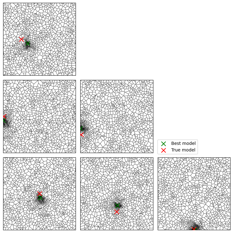
The Voronoi diagrams below show the 2D projections of the objective surface for each pair of parameters. Denser regions are more optimum (lower data misfit).
fig, axs = plt.subplots(4, 4, figsize=(10, 10), tight_layout=True)
for i in range(4):
    for j in range(4):
        if j < i:
            vor = Voronoi(searcher.samples[:, [i, j]])
            voronoi_plot_2d(vor, ax=axs[i, j], show_vertices=False, show_points=False, line_width=0.5)
            axs[i, j].scatter(best[i], best[j], c="g", marker="x", s=100, label="Best model", zorder=10)
            axs[i, j].scatter(true_parameters[i], true_parameters[j], c="r", marker="x", s=100, label="True model", zorder=10)
            axs[i, j].set_xlim(searcher.bounds[i])
            axs[i, j].set_ylim(searcher.bounds[j])
            axs[i, j].set_xticks([])
            axs[i, j].set_yticks([])
        else:
            axs[i, j].set_visible(False)
handles, labels = axs[1,0].get_legend_handles_labels()
by_label = dict(zip(labels, handles))
fig.legend(by_label.values(), by_label.keys(), loc="lower left", bbox_to_anchor=(0.5, 0.25))
<matplotlib.legend.Legend at 0x29f768990>
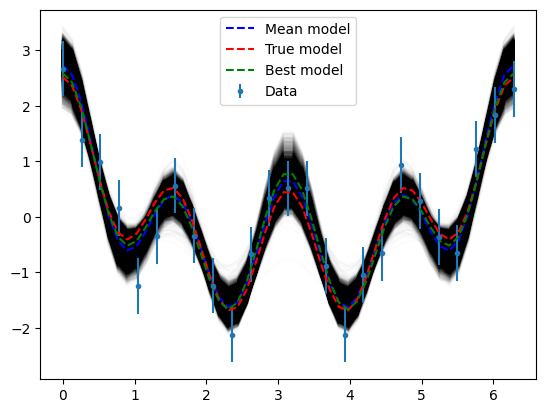
NA Appraisal Phase#
Obtain independent samples of the posterior probability density function, which is approximated from the samples obtained in the direct search phase.
A technicality here is that in the previous phase we looked to minimise the objective function i.e. minimise the predictive data misfit. In this phase we look to maximise the posterior. Under the hood, NAAppraiser expects the objective function values given to it to be the log of the posterior pdf, unless we tell it otherwise. Our objective function above is the negative log posterior
NAAppraiser with -searcher.objectives. This is done under the hood if we simply give searcher to NAAppraiser.
Note that the nomrmalisation constant is ignored because the sampler only compares ratios of posterior densities.
appraiser = NAAppraiser(
    searcher=searcher,
    n_resample=10000,
    n_walkers=10,
)

appraiser.run()
NAII - Random Walk: 100%|██████████| 1000/1000 [00:10<00:00, 92.67it/s]
NAII - Random Walk: 100%|██████████| 1000/1000 [00:11<00:00, 89.90it/s]
NAII - Random Walk: 100%|██████████| 1000/1000 [00:11<00:00, 88.49it/s]
NAII - Random Walk: 100%|██████████| 1000/1000 [00:11<00:00, 87.53it/s]
NAII - Random Walk: 100%|██████████| 1000/1000 [00:11<00:00, 86.04it/s]
NAII - Random Walk: 100%|██████████| 1000/1000 [00:11<00:00, 85.01it/s]
NAII - Random Walk: 100%|██████████| 1000/1000 [00:12<00:00, 82.28it/s]
NAII - Random Walk: 100%|██████████| 1000/1000 [00:12<00:00, 80.58it/s]
NAII - Random Walk: 100%|██████████| 1000/1000 [00:13<00:00, 73.34it/s]
NAII - Random Walk: 100%|██████████| 1000/1000 [00:14<00:00, 70.61it/s]
plt.plot(x, np.apply_along_axis(cosine, 1, appraiser.samples, mask=False).T, "k", alpha=0.01)
plt.plot(x, cosine(appraiser.mean, mask=False), "b--", label="Mean model")
plt.errorbar(xm, data, yerr=sigma, fmt=".", label="Data")
plt.plot(x, cosine(true_parameters, mask=False), "r--", label="True model")
plt.plot(x, cosine(best, mask=False), "g--", label="Best model")
plt.legend()
<matplotlib.legend.Legend at 0x12f55d610>
fig, axs = plt.subplots(4, 4, tight_layout=True, figsize=(10, 10))
for i in range(4):
    for j in range(4):
        axs[i, j].set_xlim(searcher.bounds[i])
        axs[i, j].set_xticks([])
        axs[i, j].set_yticks([])
        if i == j:
            axs[i, j].hist(appraiser.samples[:, i], bins=20, histtype="step", color="k")
            axs[i, j].axvline(true_parameters[i], color="r")
            axs[i, j].axvline(appraiser.mean[i], color="b", linestyle="--")
            axs[i, j].axvline(best[i], color="g", linestyle="--")
        elif j < i:
            axs[i, j].scatter(appraiser.samples[:, i], appraiser.samples[:, j], s=0.5, color="k", alpha=0.1)
            axs[i, j].scatter(true_parameters[i], true_parameters[j], color="r", marker="x")
            axs[i, j].scatter(appraiser.mean[i], appraiser.mean[j], color="b", marker="x")
            axs[i, j].scatter(best[i], best[j], color="g", marker="x")
            axs[i, j].set_ylim(searcher.bounds[j])
        else:
            axs[i, j].set_visible(False)
